Making Sense of the Digital Deluge

Clustering Content from the Web

How do we at Continua choose what goes into your podcast? It’s a three-phase process. Based on your podcast preferences, we first scrape the web and extract relevant information. Next, we rank extracted content based on whether it will be interesting to you. Finally, we cluster that content, and these clusters form the basis of your podcast sections. Today’s post is going to focus on that final step.

Given a plethora of webpages that have been deemed interesting to you, we want to present that information in a coherent way. We can’t simply dump all the content into a prompt and ask an LLM to create you a podcast, because we’ll likely hit context window limits. Research has also shown that incredibly long prompts can negatively impact the capabilities of LLMs. Instead, we need to pick the most compelling content and segment it so that each call to the LLM does not exceed the context window. How do we segment the data? We cluster it.

We can’t throw all our content into a single prompt and ask the LLM to create a podcast. This will likely cause us to exceed context window limits and potentially diminish output quality. Instead, we cluster the web content into semantically similar pages and pass each cluster through an LLM independently.

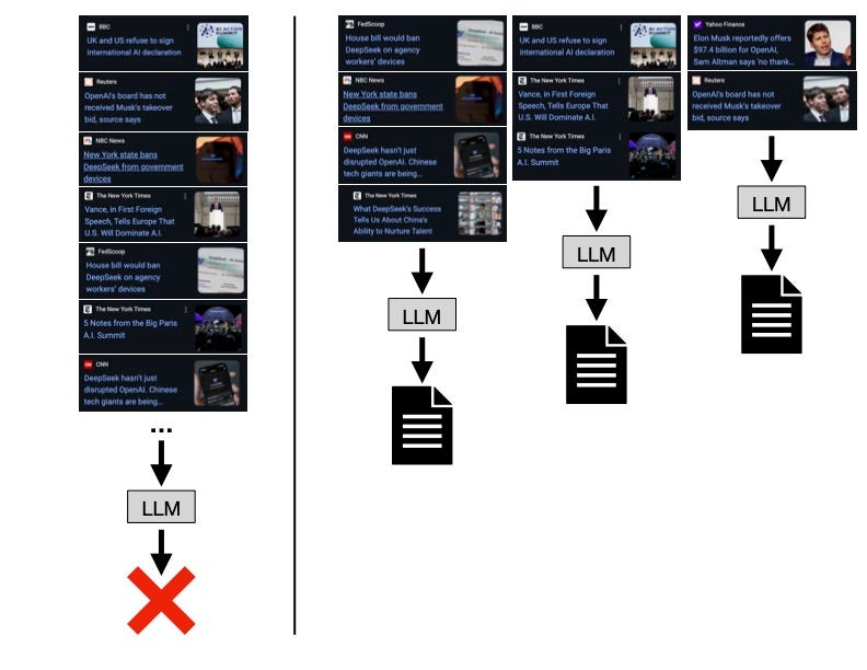
Clustering is the process of grouping together objects that are similar, while distinguishing objects that are different. Realistically, the same content is likely to be covered by many media sources. The publications may have different spins or contain slightly different details, but at their core, they cover the same story. Ideally, those stories would be grouped together, so that in a single call to the LLM, we ask it to present the information on one subject. In this way, we prevent your podcast from covering the same content in multiple sections and simplify the task for the LLM, resulting in a higher quality output.

Generating Embeddings

Before we can cluster our documents, we must first transform the raw text into high-dimensional embedding vectors, which capture the semantic meanings of the documents. Models that generate embeddings are trained so that documents covering similar concepts are “closer” to one another in the embedding space. We define “closeness” as cosine similarity, or the cosine of the angle between two vectors. Intuitively, two vectors pointing the same direction will have a cosine similarity of 1, indicating maximum similarity; two vectors orthogonal to one another will have a cosine similarity of 0, indicating no similarity; and two vectors pointing in opposite directions will have a cosine similarity of -1, indicating maximum dissimilarity.

Agglomerative Clustering

Once we have embeddings, we need to segment the data into meaningful sets. Many different algorithms exist for clustering: among others, some partition the data into a pre-defined k clusters, some group the data based on the density of points, and some take a hierarchical approach, creating a tree of nested clusters. We avoid the first class of methods, since we want a variable cluster count. It makes little sense for us to force k clusters, when we don’t know ahead of time if our documents will cover a single subject or many. For instance, we wouldn’t want to force documents covering 10 semantically different topics into 5 clusters arbitrarily. We experimented with both density-based clustering, as well as hierarchical clustering, and settled on the latter, specifically agglomerative clustering. Agglomerative clustering starts with each data point as its own cluster and iteratively merges clusters together until all points are in a single cluster. Two clusters are merged based on a linkage criterion that determines whether they are “close enough” to one another. The linkage criterion can minimize the variance of the sets being merged, the average of distances between each pair of observations in the two sets, the maximum distance between any two observations in the two sets, or merge the sets that have the minimum of the distances between all observations in the two sets. The algorithm can be stopped early: either once there are k final clusters or all clusters are beyond some distance threshold from one another. We choose the latter approach, since we don’t want to always force k clusters. Unfortunately, we cannot choose a static distance threshold, since each batch of documents we cluster are likely to be differently distributed in space.

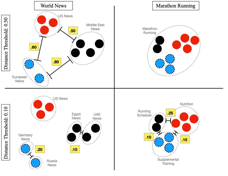
Imagine that we have one batch of documents covering various topics in world news, and there are clear clusters corresponding to US news, European news, and Middle East news. The distance threshold between these clusters may be quite high, as they’ll be covering quite distinct topics. Now, imagine that we have a batch of documents all discussing training for a marathon. These are likely to be much closer to one another in embedding space, but perhaps the best podcast would result if we were able to segment these documents based on different aspects of running, including nutrition, run schedule, and supplemental training. If we apply the same distance threshold for the marathon training podcast as we do for the news podcast, these documents are likely to end up in a single cluster. If we go the other direction, our world news podcast will cover more specific local stories, instead of providing an overview of news from each global region. Therefore, we need a way to define an adaptive distance threshold based on our current batch of embeddings.

Different batches of web content will have drastically different distributions in space, motivating the need for an adaptive distance threshold in agglomerative clustering. If we had the same threshold for every data batch, we would cluster things in a less than ideal way, as shown above.

In order to find the best distance threshold for a given batch of embeddings, we do a parameter search over the distribution of distances between points in our current batch, and choose the distance threshold that results in clusters that maximize average silhouette score. Silhouette score is a metric that balances the relationship between average intra-cluster distance and the average nearest-cluster distance, with the best score being 1 and the worst being -1. We exclude clusters with only one member from the silhouette score calculation.

Pruning Our Clusters

Once we have our final clusters, we have to choose which make the final cut for podcast generation. Let’s say we have a target value of y clusters for podcast generation. If our clustering process returns fewer than y clusters, we proceed to generation with limited content. More often, our clustering process returns many more than y clusters and we have to downsample. Recall that all documents were previously ranked based on perceived user interest. As a result, we can calculate an average rank per cluster and return the y clusters with the highest average user interest scores.

However, the process does not stop here. Even within a single cluster, we can have way too much textual information, forcing us to downsample further. We prune our final within-cluster documents based on both individual document rank and source. We believe that the best podcasts will not only cover the most interesting documents, but also documents from diverse, trustworthy sources. For example, instead of a podcast segment covering 10 articles from CNN, we believe a better listening experience comes from a segment based on articles sampled from CNN, BBC, and NPR. Given a cluster with N total documents from m sources, we assign a probability to each of the N documents based on how many documents come from each source. This probability is adjusted to account for the assumption that a higher volume of stories are likely to come from more reputable sources.

After all of that, we have the final content that will be used to generate a podcast! Come back next week to learn about the process of podcast transcript creation!